Introduction to sequence analysis in R

In this post we will look at how to read, write and analyse fasta sequences in R using the ape, pegas and phangorn libraries.

We will go through a few example analyses to get you started.

Example sequence and data files are available in the sequence-gazing repo here in Example_fasta and Example_data directories.

Let’s start by reading our small example alignment of fasta sequences into R, we can use the function read.dna() to do this, which will read our fasta file and create a “DNAbin” object:

alignment <- read.dna("example.fasta", format = "fasta")

We can check the class of our object by using R’s inbuilt class() function:

class(alignment)
[1] "DNAbin"

If we call the alignment in the Rstudio console we should see the following summary information:

Now that we have read our DNA data into R we can use the many functions available for sequence analysis. Let’s try a few out!

Example 1

We can calculate the nucleotide diversity using nuc.div() , haplotype diversity using hap.div() and GC content using GC.content() for our alignment.

nuc.div(alignment)
[1] 0.005649718

hap.div(alignment)
[1] 0.8666667

GC.content(alignment)
[1] 0.3276836

Example 2

We can also build and plot a quick phylogenetic tree from our data.

First let’s find the best fitting substitution model for our sequences using modelTest from the phangorn library.

Note that to use the modelTest function we need to convert our DNAbin object to a phyDat object using the function phyDat().

In this example we are testing all available models including models with varying G (gamma) and I (invariable sites):

model_test<-modelTest(phyDat(alignment), G=TRUE, I=TRUE, model="all")
best_fit_model <- as.pml(model_test)

Using as.pml() we can find the best fitting model from the model fitting analysis.

Below we can see the model that best describes the molecular evolution of our sequences is the F81, note that I and G are not displayed, meaning the best fitting model did not include gamma or invariable site information.

We will cover substitution models in more detail in another post, for now let’s use this information to build a quick tree from our distance matrix.

First we use dist.dna() to create the DNA distance matrix, specifying the substitution model as F81.

dist_matrix <- dist.dna(alignment, model = "F81", as.matrix = TRUE)

Now we can build the tree using the Neighbour-joining algorithm.

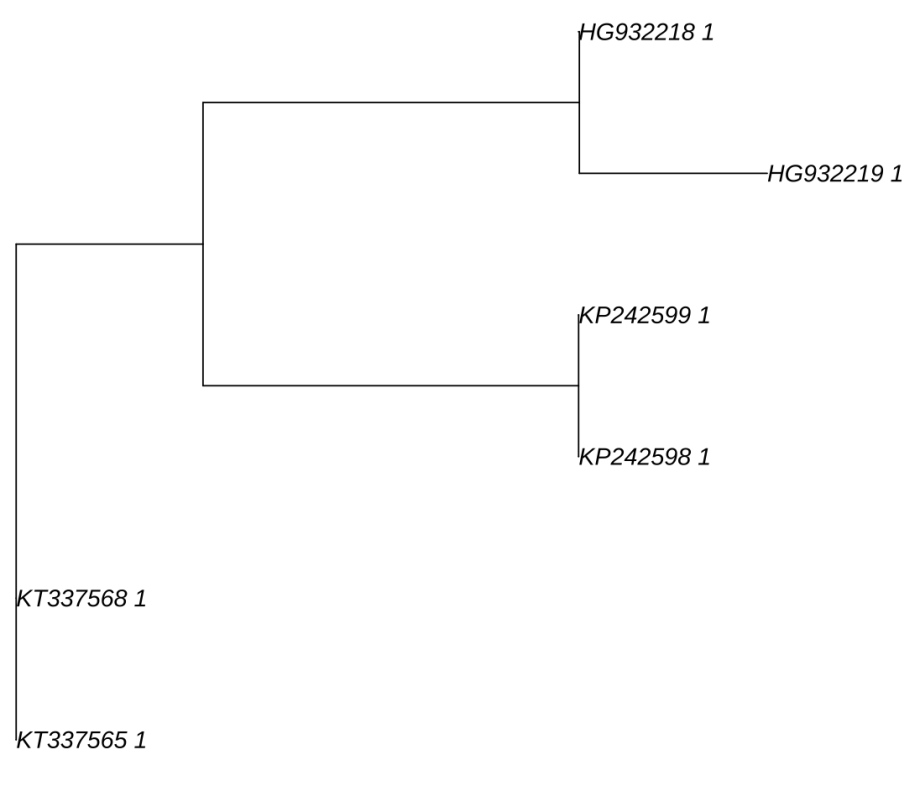
NJ_tree<-nj(dist_matrix)
plot(NJ_tree)

Try it out, your tree should look like this!

Example 3

If we want to incorporate additional information into our sequence analyses such as geographic locality, measurements or some other group category we can supply a csv file with associated information for each sequence (we also call this metadata).

Let’s read in our metadata as a csv file:

metadata<-read.csv("example_metadata.csv", header=TRUE)

Our metadata table looks like this:

   Accession Locality Group
1 KT337565.1       UK     1
2 KT337568.1       UK     1
3 KP242599.1   France     2
4 KP242598.1   France     2
5 HG932219.1    Italy     3
6 HG932218.1    Italy     3

There are many things we can do with this metadata.

For now imagine we want to extract the sequence data belonging to a certain group, let’s say group 1:

We can start by subsetting our csv table by the “Group” column using the subset() function:

group1_ids <- subset(metadata, Group == "1")

In our alignment, as it is a DNAbin object , the rownames are the sequence Accession ids:

We can extract the sequences associated with group 1 based on these Accession ids :

extracted_sequences <- alignment[rownames(alignment) %in% group1_ids$Accession,]

Now that we have our sequence entries stored in our new variable we can run some other analyses or write out the data for later:

We can use write.dna() to write our data to a fasta file with the standard 60bp per line format:

write.dna(extracted_sequences, file = "group1.fasta", format = "fasta", colsep = "", colw = 60, nbcol=1)